How to Download and Interpret GHCNm Monthly Station Data

Follow a reproducible workflow to select a NOAA GHCNm station and month, export its CSV history, check quality fields, and calculate a linear trend.

Author

Climate Explorer Team

Modified

August 27, 2026

Open the interactive GHCNm station explorer

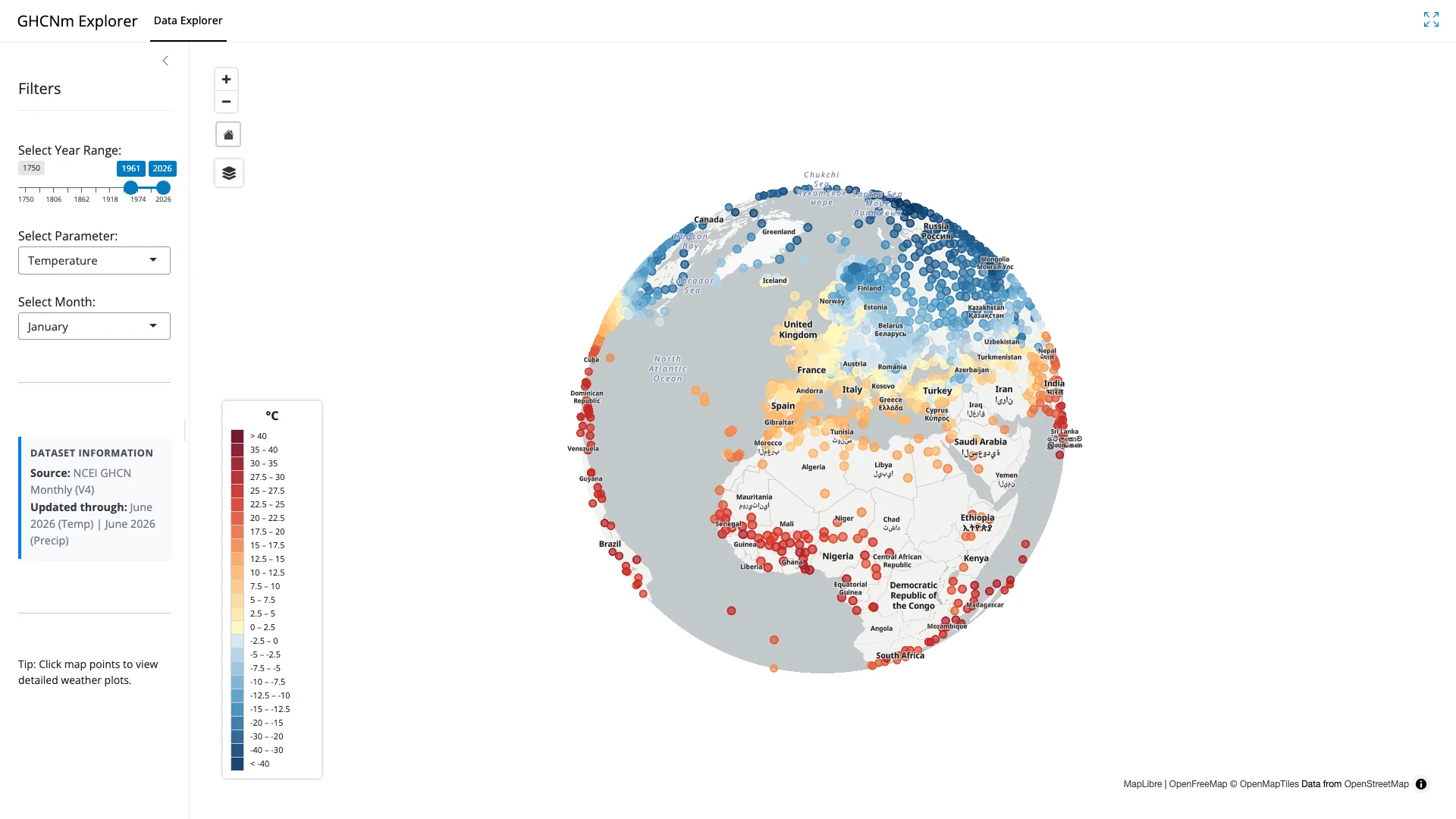
GHCNm explorer global map with colored station markers and controls for year range, parameter, and calendar month — GHCNm Explorer map showing the global monthly station network

Quick start

Open the Explorer and choose Temperature or Precipitation.
Choose one calendar month and a year range.
Zoom to a station and click its marker to open the station plot.
Inspect gaps, flags, and the fitted trend before using the result.
Select the download icon below the plot to export the active station-month series as CSV.

1. What this workflow produces

The GHCNm Explorer is an independent Climate Explorer interface for records maintained and published by the NOAA National Centers for Environmental Information (NCEI). Climate Explorer is not affiliated with or endorsed by NOAA. NOAA/NCEI remains the authoritative source for the archive, station metadata, quality-control methods, and revisions.

Following this guide produces one CSV containing the selected station, parameter, calendar month, and year window. This is useful for a reproducible station-history calculation because the export preserves the years and values used by the plotted linear trend. It does not produce a national, regional, or global average.

2. Know which series the Explorer serves

The two Explorer choices come from different GHCNm products and should not be interpreted as if they received the same processing.

GHCNm series currently served by the Explorer
Explorer choice	Series served	Unit	Important interpretation
Temperature	NOAA GHCNm v4 monthly mean temperature (`TAVG`) from the quality-controlled, adjusted `qcf` archive	°C	NOAA applies the Pairwise Homogenization Algorithm (PHA) to this adjusted product. The Explorer does not currently offer the unadjusted `qcu` series or monthly minimum/maximum temperature.
Precipitation	NOAA GHCNm v4 monthly precipitation, currently published by NOAA as a beta product	mm	These are monthly totals and are not PHA-adjusted. Coverage and source fields differ from temperature.

NOAA also publishes quality-controlled unadjusted temperature (qcu). Use the NOAA archives in Section 7 when the analytical question requires an adjusted-versus-unadjusted comparison. Do not describe a Climate Explorer temperature plot as “raw”: the displayed temperature series is the adjusted qcf product.

3. Select a comparable station history

Step 1: Choose the parameter and month

Select Temperature or Precipitation, then choose one calendar month. The chart compares that same month across successive years—for example, January with January—not all twelve months in sequence.

Step 2: Set the year range

Use Select Year Range to define the analysis window. The map retains stations whose metadata span the requested endpoints, but that does not guarantee a value for every intervening year. A station can still contain gaps.

For a first trend inspection, prefer a window of several decades. Then move the start and end years to see whether the fitted slope is sensitive to the chosen period.

Step 3: Select the station

Zoom to the location and click a station marker. The popup identifies the station name, GHCNm ID, elevation, available years, selected years, and the multi-year mean for the active calendar month. Use the station ID—not only the displayed name—when documenting or repeating the analysis.

Home button: Return the map to the global station view.
Layer control: Change the basemap or turn place labels on and off.
Full Screen View: Click the Maximize / Full Screen button in the top-right corner of the explorer window to expand the dashboard to full display size. This is recommended when inspecting complex multi-panel charts, high-density station maps, or large data tables. Press Esc or click the icon again to exit.

4. Read the station plot before downloading

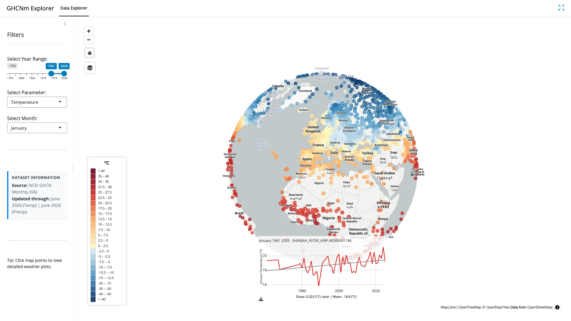
GHCNm station panel with yearly values for one selected calendar month, a gray linear trend line, slope and mean labels, and a CSV download control — GHCNm explorer station panel showing a monthly temperature series and fitted linear trend

The red or blue line shows the available monthly values for the selected station and calendar month. Missing years break the observed line rather than being treated as zero. The gray line is an ordinary least-squares linear fit of VALUE against YEAR for the active selection.

The displayed slope is a descriptive rate for one station, one variable, one month, and one selected period. It does not by itself establish statistical significance, identify a cause, or represent a whole country. Before drawing a broader conclusion:

Look for gaps and isolated values.
Test at least one reasonable alternative start or end year.
Compare nearby stations with overlapping records.
For temperature, compare NOAA’s adjusted and unadjusted products when adjustment sensitivity matters.
Use a regional dataset and uncertainty analysis for regional or global claims.

For the scientific reasoning behind these checks, read what a GHCNm station trend can—and cannot—show.

5. Worked example: Heathrow January temperature

This example creates an export that can be checked against the station trend shown in the related article.

Open the GHCNm monthly station explorer.
Set Select Parameter to Temperature.
Set Select Month to January.
Set the year range to 1961–2025.
Zoom to southeast England and select HEATHROW, GHCNm station ID UKM00003772.
Confirm that the plot title identifies January, the selected period, Heathrow, and the station ID.
Select the download icon beneath the plot. The filename includes the station name, station ID, and month.

The Explorer uses the currently loaded NOAA release. A later upstream revision can change individual values or the fitted slope, so record the download date when using the result in research or publication.

6. Check and reproduce the CSV result

Temperature export fields

Temperature columns in the Explorer CSV
Column	Meaning
`ID`	Eleven-character GHCNm station identifier
`YEAR`	Calendar year
`ELEMENT`	`TAVG`, monthly mean temperature
`MONTH`	Numeric calendar month, 1–12
`VALUE`	Adjusted monthly mean temperature in °C
`DMFLAG`	NOAA data-measurement flag
`QCFLAG`	NOAA quality-control or adjustment flag; a blank field does not mean the entire station history is error-free
`DSFLAG`	NOAA data-source flag

Precipitation export fields

The precipitation CSV includes station metadata alongside the monthly totals and upstream flags. In the current Climate Explorer preprocessing, trace precipitation encoded upstream as -1 is represented as 0 mm; rows carrying the configured failed-quality codes are excluded before display. Preserve the remaining fields when exporting so the source and measurement context are not lost.

Precipitation columns in the Explorer CSV
Column	Meaning
`ID`	Eleven-character GHCNm station identifier
`station_name`	Name of the station
`latitude` / `longitude` / `elevation_m`	Station location coordinates and elevation in meters
`YEAR`	Calendar year
`MONTH`	Numeric calendar month, 1–12
`precip_tenths_mm`	Original precipitation value in tenths of a millimetre
`VALUE`	Precipitation total in mm
`measurement_flag`	NOAA data-measurement flag
`quality_flag`	NOAA quality-control flag
`source_flag`	NOAA data-source flag
`source_index`	NOAA source index

Recalculate the fitted slope in R

Replace the filename below with the downloaded file. This calculation reproduces the Explorer’s basic linear model for the exported rows; it is not a complete uncertainty analysis.

d <- read.csv("HEATHROW_UKM00003772_January.csv")
d <- subset(d, is.finite(YEAR) & is.finite(VALUE))

missing_years <- setdiff(seq(min(d$YEAR), max(d$YEAR)), d$YEAR)
fit <- lm(VALUE ~ YEAR, data = d)

missing_years
unname(coef(fit)["YEAR"])
mean(d$VALUE)
table(d$QCFLAG, useNA = "ifany")

Report the station ID, parameter, calendar month, start and end years, number of available values, slope unit, and download date. If years are missing, report that too.

7. Source archives and adjusted versus unadjusted temperature

NOAA GHCNm dataset overview: Product scope, methods, documentation, and precipitation status.
GHCNm v4 temperature archive: Current qcf adjusted and qcu unadjusted temperature packages.
GHCNm v4 temperature readme: File layout, units, and definitions of QCU, QCF, DMFLAG, QCFLAG, and DSFLAG.
GHCNm v4 source-flag definitions: Origin represented by each temperature source flag.
GHCNm v4 precipitation archive: Source precipitation packages.

Use qcf when the goal is to inspect NOAA’s adjusted monthly mean temperature series. Use qcu from NOAA when the goal is to see how the unadjusted quality-controlled observations differ. A difference between the two is evidence of an applied adjustment, not proof of the physical cause of the discontinuity. Station metadata and neighboring records remain important.

8. Troubleshooting and limits

No station marker remains: Shorten the requested year span or switch the parameter; temperature and precipitation have different station coverage.
The selected station has no plot: Try another calendar month or a shorter period. Metadata coverage can span the endpoints even when the chosen month contains no usable values.
The chart contains gaps: Treat them as missing observations, not zero. Check the CSV before fitting or comparing trends.
The fitted slope changes: Record the selection and test sensitivity to the time window. A linear fit is only a summary of that chosen period.
You need unadjusted temperature: Download NOAA’s qcu product; the Explorer currently serves only adjusted qcf monthly mean temperature.
You need daily or hourly events: Use the GHCNh hourly-data workflow or another higher-frequency source. Monthly GHCNm data cannot resolve the timing of individual weather events.